3D Rendering Engine and Robot Kinematics Simulation
A write-up on the robot kinematics simulation (and accidental software renderer) I made, exploring forward and inverse kinematics, Denavit-Hartenberg parameters, and practical applications on a physical robotic arm. Way too much math in this one :(
3D Rendering Engine
Objective
The 3D rendering engine, built in Python, utilizes pygame to render pixels on the screen and homogeneous transformation matrices to represent affine transformations in the ambient space. Used as the environment in which inverse kinematics with a robotic arm will be explored. Additionally supports dynamic mesh rendering and custom script support to subscribe to an update loop.
Posing Features
This section delineates the classes/components used in the engine to represent position and orientation in .
RotationMatrix Class
General Purpose
This class serves as a representation of rotation in the ambient space. Taking a roll, pitch, and yaw as parameters (stored internally as a 3x3 numpy matrix), the class provides the user with a packaged representation of rotations, which are a member of the Lie group (Special Orthogonal Group), the group of rotation matrices about the origin in .
Euler Angles
For ease of user instantiation, rotation matrices take a roll about the x-axis, a pitch about the y-axis, and a yaw about the z-axis, then convert them to a final rotation matrix by successively applying each axis of rotation. If the roll matrix is , pitch , and yaw , the final rotation matrix is found as Where the order of multiplication is standard convention for Euler angle representations. While Euler angles might suffer from gimbal lock in specific rotations, they are sufficient when considering a differential rotation, so they are a usable representation in this project. A more robust 3D engine might consider implementing quaternions instead to combat this issue.
Matrix Operations
Full support for matrix-matrix and matrix-vector multiplication, matrix inversion, and operator overloading for ease of usage in other mathematical operations (matrix multiplication included).
Vector3 Class
General Purpose
This class serves as a representation of position in the ambient space. Containing an , , and coordinate (internally stored as an numpy array), the class provides the user with a packaged representation of 3-vectors.
Homogeneous Coordinates
While a 3-vector is sufficient to represent position in , appending a component to the vector allows for affine transformations in conjunction with transformation matrices.
Vector Operations
Full support for 3-vector inner products, wedge products, and operator overloading for ease of usage in other mathematical operations (matrix multiplication included).
Skew Symmetric Matrices
In conjunction with the RotationMatrix class, the Vector3 class can represent itself as a rotation matrix through skew symmetric matrices. Defined as a matrix where , the skew symmetric matrix can also represent the cross product operator with a specific vector, defined as
for some vector . More importantly, this matrix is a member of , the Lie algebra of (it can be pictured as the tangent space of at the identity). Thus, because a Lie algebra can be taken to its corresponding Lie group through matrix exponentiation (logarithm for the reverse), we can compute the corresponding rotation matrix in . For exponentiation, we utilize Rodrigues’s Formula: letting us quickly obtain a rotation matrix equivalent to rotating around the unit axis .
Transform Class
General Purpose
This class serves as a representation of affine transformations in the ambient space. Taking advantage of both the RotationMatrix and Vector3 classes, the class provides the user with a packaged representation of transformation matrices, which are a member of the Lie group (Special Euclidean Group), the group of transformation matrices in .
Representation
Transformation matrices are defined as where and . By pre-multiplying by a transformation matrix, the rotation then translation is applied to the following homogenous 4-vector or following transformation matrix, similar to how pre-multiplication by a rotation matrix applies the rotation. The Transform class internally stores a transformation matrix, separating out positional and rotational information as the user requests it.
Child Hierarchy
Each transform possesses 1 parent and children, as well as a local transformation matrix representing its pose in the parent frame. When a transform’s position or rotation is updated, each child is recursively updated, effectively moving the child with the parent frame, along with any children of children, by applying this transformation to every child: where primes denote the homogeneous transformation matrix after the updated pose, and all transformation matrices are in the global frame (standard basis). We take advantage of the fact that local coordinates do not change if a parent moves to preserve that value.
Twists
A twist is defined as which represents an affine transformation with angular velocity and linear velocity . A normalized twist, or screw , is defined as where is some scalar displacement that represents motion along the screw axis (both rotation in radians or linear translations). In this implementation, twists and screws are utilized to achieve rotation and translation about a screw axis. To avoid using a 6-vector and for ease of computational implementation, can also be written as a matrix, a member of the Lie Algebra of , represented as where and . If normalized to be a screw, premultiplication by this matrix represents an infinitesimal affine transformation. similar to how skew-symmetric matrices represent infinitesimal rotations. Thus, we use these twists to apply an affine transformation on a transformation matrix through matrix exponentiation. In a screw matrix, is expressed as the linear velocity in the plane of rotation defined by the bivector of rotation. We can calculate this linear velocity using a local transform’s offset from the point of rotation as follows: Where is the offset from the point of rotation and is the angular velocity about the point of rotation.
Given a reference frame , unit angular velocity , and unit linear velocity , where and is the left Jacobian of , which is necessary to correct the velocity relative to the simultaneous rotation. This can be written in a closed form as The Transform class supports two abstracted transformations for ease of use when programming classes for a desired simulation: rotation around a specified axis by some angle and translation in a specified direction by some distance. Both methods utilize premultiplication by a twist matrix to cleanly update the stored transformation matrix in the class.
Adjoint Representation
When attempting to change the basis of a twist six-vector, we cannot merely pre-multiply by a transformation matrix due to the dimensional mismatch. Thus, we utilize the adjoint representation of instead. Given a transformation matrix with rotation component and position component the adjoint representation is
Pre-multiplying by the adjoint representation in six dimensions is equivalent to premultiplication by a transformation in four dimensions, so using this, we can effectively apply a transformation to a twist six-vector.
Simulation Features
This section is an overview on the classes/components used in the engine to maintain an update loop that simulate real-time akin to reality.
Engine Class
General Purpose
This singleton class controls the update loop of the game engine, refreshing the state of the game every frame to discretely simulate real life. This class subscribes to Updater classes (see below) to discern what behaviors to invoke each frame. Additionally, it controls the engine frame rate (and delta time) and also maintains a reference to the SceneRenderer class that is responsible for redrawing the camera view.
Updater Class
General Purpose
This inheritable class is used to connect to the Engine’s update loop. Classes which extend this class are provided with different methods which the Engine subscribes to, allowing for dynamic gameplay. These methods include:
awake(): Called once upon instantiation of an Updater. Used for initial setup.
start(): Called once upon instantiation of an Updater after every awake() method is called during the frame. Used when initialization is dependent on other Updaters.
update(): Called once per frame for each Updater. Houses the general logic associated with an Updater that governs its behavior during the update loop.
late_update(): Called once per frame for each updater after every update() method is called during the frame. Used to delineate any behavior that is dependent on the processes that occur during the frame.
As a result, all objects that exist in the game view should be tied to an updater so they are recorded by the engine and renderer.
Component Structure
For ease of scalability, Updaters should act as the primary containers for any additional components that may exist on the object. For example, meshes, cameras, lights, and any custom-made component should all exist as a reference tied to an extended Updater class. In the scope of our robotic arm, we utilized a custom Updater class called CameraController to provide camera navigation to the user through keyboard input.
Rendering Features
This section covers the classes/components used to translate poses in to screen space such that it can be viewed on a typical monitor.
Camera Class
General Purpose
The Camera class determines what is visible from the game view. While not an Updater class, instead acting as an additional component with an innate transform. The camera class maintains an aspect ratio, a FOV, a near-clip plane, and a far-clip plane to apply a perspective projection to determine what to render.
Perspective Projection
When computing the screen coordinate that corresponds to a homogeneous coordinate , we utilize pre-multiplication by a perspective projection matrix . This matrix must account for the camera’s current orientation and position, then project a point between the near and far clip plane to screen coordinates. Thus, we separate into a view component and projection component such that Notably, this matrix does not directly take the homogeneous coordinate to the screen space, but first to a clip space vector such that Through this clip space vector, we can then convert to a normalized device coordinate through the following nonlinear transformation: This transformation will result in a normalized device coordinate that is scaled to always range between and . As a result, if the screen has height and width , providing us with a method to convert from homogeneous coordinates to screen space through simple operations. Note that the z component in this situation is not used, but in our implementation of this function, we additionally return to encode depth in normalized device coordinates.
Computing the View Matrix
To compute , we must define , a transformation matrix that when pre-multiplied, rotates a point to the camera’s orientation, then shifts the point such that the camera is at the origin, performing an affine transformation where the camera resides at the new origin.
To construct this, the camera provides its position , as well as a target position that the camera is facing toward. Finally, it also provides a vector pointing in the "up" direction as seen by the global frame (if the camera were facing the z-axis, for instance, would point in the y-axis). Through this, we can use a partial version of the Gram-Schmidt orthonormalization process to generate an orthonormal basis of the camera’s reference frame. First, we calculate the forward vector such that the right vector such that and a new up vector (we must calculate a new up vector to preserve orthonormality in all cases due to occasional floating point error) such that It is important to note that we could provide the right vector and undergo the same process, but we begin with the up vector to preserve a convention. Thus, we can construct as Notably, we must negate to represent the vector direction from the target to the camera, as represents the opposite. Additionally, the final column of encodes the translation necessary to shift the camera to the origin, represented through negative dot products between the orthonormal basis and the camera’s position. As a result, pre-multiplication by transforms a homogeneous coordinate to the orthonormal basis of the camera’s reference frame.
Computing the Projection Matrix
Next, we must construct a matrix that projects a homogeneous coordinate in the camera’s orthonormal basis to clip space, mapping the view frustum to a canonical viewing volume, which we choose to be a rectangular prism with half-extents and center (we choose this definition instead of a symmetrical cube to simplify calculations in the future). In clip space, the coordinates are scaled such that it preserves depth information through a nonlinear transformation.
To understand how the projection matrix operates, we will inspect each of the four components of view-projected homogeneous coordinate where to convert to clip space coordinate such that First, we inspect the y-component. We can scale this to clip space through the vertical field of view (), representing the angle that describes how wide the camera can see, from the bottom view plane to the top view plane. Thus, we can calculate scaling factor as so Because the field of view is defined vertically, to calculate the x-component, we need to adjust for a non-square screen, which can be done through the aspect ratio, the proportion of width to height. Thus,
Next, we must inspect the w-component, the homogeneous element. Recall that after applying perspective projection, we normalize by a final time before rendering it on our camera, achieving such that When we apply this normalization, the effect we wish to achieve is a scaling of and such that objects further away are rendered comparatively smaller. Therefore, to achieve this effect, we want to vary negatively with , so
Finally, when transforming the z-component, we must provide a notion for the distance where our camera starts and stops rendering so we can effectively convert depth to coordinates within a given range. Thus, we must define near clip plane and far clip plane to denote these distances. Because the camera looks in the negative z-direction, we wish to find a mapping such that and Because should not depend on or , we guess that where we wish to solve for some and that satisfy the previously stated condition. Applying the boundary conditions, we obtain and which we can solve to obtain and Thus, by combining the respective transformations for each component, we can express everything as a final projection matrix of
Mesh Class
General Purpose
The Mesh class depicts a three-dimensional mesh constructed of vertices (coordinates in ) and edges (indexed pairs of vertices). Through this, the SceneRenderer can render these meshes as a wireframe through perspective projection. Additionally, the Mesh class can compute faces (indexed triples of vertices) through the edge list, along with storing associated colors for rendering. The Mesh class can also read .obj files, which encode vertex positions and mesh triangles within the format.
Edge-Face Conversions
To calculate a list of faces from a set of edges, the Mesh class supports face detection. Because our list of edges is a finite graph, we can construct an adjacency matrix that fully represents our mesh. Next, we first iterate over each vertex, then over each vertex’s subgraph of neighbors, utilizing a stack to keep track of traversed vertices. If we return to the original vertex at any point, we have discovered a cycle, hence found a face, which we can add to a preexisting set of faces. It is important to also provide a max cycle length as well to avoid infinite loops. Upon completion of this process, we will have obtained the set of all faces present on the mesh within a certain cycle length.
We can run this process in reverse to generate edges from faces as well, by simply adding each edge in the face cycles to a set of edges. This method is useful to save computation time when provided with a .obj file and a wireframe render is desired.
Triangulation
To support efficient mesh rendering, the Mesh class also automatically triangulates all faces present in the mesh, assuming that all faces are simple polygons. To triangulate a face, we first distinguish between convex and concave polygons, depicted in Figure 1. Convex polygons are those with interior angles less than 180 degrees. As a result, we can triangulate these faces by selecting an arbitrary vertex and connecting it to every other vertex in the face by adding an edge. Thus, in linear time, for an -gon with edges, we add edges to our set of edges and convert our one face to faces.
To detect whether a face is convex, we take advantage of the fact that the enclosing contour of a convex polygon always curls in the same direction at any vertex. In other words, if you selected a vertex and began traveling clockwise, you would continue traveling clockwise until you reach the starting vertex without ever traveling counter-clockwise. Thus, we compute the cross product between the edges next to each vertex, and if every computed cross product returns the same direction, we can infer that the face is convex.
To triangulate a concave polygon, we utilize the ear clipping method. Consider three consecutive vertices , , and such that is a convex vertex (determined through the previously described convexity method). As such, the edge between and must enclose a triangle within the overall polygon. If the triangle does not enclose any other vertices, we can "clip" this "ear" of the polygon by connecting these two vertices. As a result, we obtain a new polygon with which we can iterate this process until we obtain only triangles, giving us a possible arrangement of subdivisions to triangulate our polygon. This process is demonstrated in Figure 2.
SceneRenderer Class
General Purpose
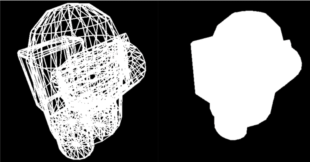
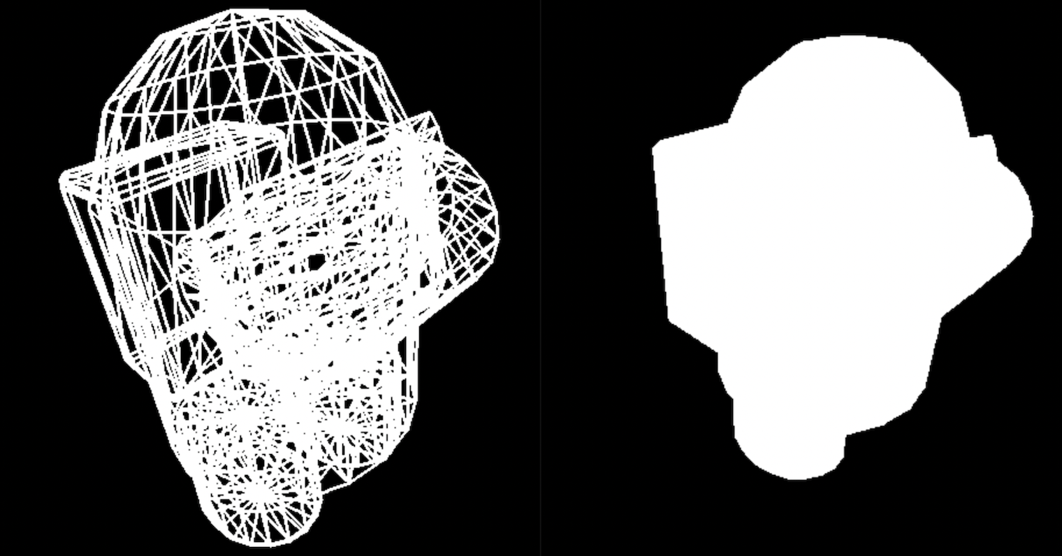
The SceneRenderer class is responsible for rendering anything seen by the camera to the screen, converting a continuous range of coordinates to discrete screen pixels, along with rendering objects closer to the camera in front of further ones. Furthermore, it must run efficiently, as it must refresh the screen at a frame rate that appears continuous to our eyes. To accomplish this, we utilize a depth buffer to order entities in the ambient space for fast rendering. An example render is shown in Figure 3.
Occlusion Culling
To render meshes on the screen, the SceneRenderer employs occlusion culling using a depth buffer to manage the relative distances between meshes and the camera, enabling computationally efficient rendering. Every frame, the SceneRenderer iterates over every active mesh in the scene (all meshes linked to an Updater) and attempts to draw every face. Because our Camera class also returns the distance to the camera when projecting vertices to screen space, when rasterizing, we can track each individual pixel’s distance to the camera and only render the pixel on the mesh closest to the camera. As a result, we prevent ourselves from unnecessarily rendering obscured objects. Finally, we utilize a screen blit (block image transfer) to transfer a 2-dimensional array representing desired color values to the actual screen. The combination of these two methods greatly save on computation time, something that is necessary when running a frame-based engine.
Depth Buffers vs. Sorted Buffers
It is important to distinguish between different ways of quantifying distance to the camera. Our renderer utilizes a depth buffer to most accurately track each individual pixel’s distance to the screen, which accounts for overlapping meshes in the scene. An alternative approach would be using a sorted buffer, which instead computes the depth face-by-face by taking the average of the vertices’ camera distance. While this approach is less computationally heavy, removing the need to utilize barycentric coordinates (see the following section), we face an unexpected downside. Depending on subtle camera orientation fluctuations, meshes that obscure others will tend to flicker back and forth as the average depth changes. As a result, while certain orientations render as expected, others will fail to do so accurately, an issue that is especially apparent with a free-look camera. As such, we utilize a depth buffer for the purposes of this project.
Barycentric Coordinates
Barycentric coordinates provide a convenient way to express points relative to the vertices of a triangle. Let a triangle have vertices Any point in the plane of the triangle can be written as a convex combination of the vertices: subject to the constraint A point lies inside the triangle if and only if The barycentric coordinates also serve as weights for linear interpolation of any per-vertex quantity, such as depth, color, or normals. For instance, the interpolated depth at point is
Line Rasterization
Line rasterization proceeds by sampling points along a line segment connecting two screen-space vertices. Let The line is parameterized by Pixels are generated by evaluating at discrete intervals proportional to the Euclidean distance For lines of finite thickness, neighboring pixels within a given radius are also considered. Each candidate pixel’s depth is compared to the depth buffer, and the pixel is drawn if it is closer than the current buffer value. Once this test passes, the pixel is assigned the specified line color.
Triangle Rasterization
Triangle rasterization uses barycentric coordinates to determine pixel coverage and interpolate attributes. Let the triangle vertices be A pixel at screen-space location is considered inside the triangle if its barycentric coordinates , computed using the areas of sub-triangles or edge functions, satisfy The barycentric coordinates allow linear interpolation of vertex attributes. In particular, the pixel depth is interpolated as which is then incorporated into the depth buffer for visibility. Similarly, barycentric coordinates can interpolate color, normal vectors, or texture coordinates, enabling smooth shading and other per-pixel effects.
Robotic Arm
Objective
Replicate the behavior of a four-jointed robotic arm in the aforementioned 3D rendering engine. Utilize inverse kinematics to control the arm’s end effector to reach different target poses for simple tasks. The final goal is to remove a 1/4-20 nut from a bolt and relocate it to a different bolt.
Implementation
Joints
Features
The Joint class extends Updater, providing it with a world transform and access to the main update loop of the engine. Joints also possess an axis of rotation (defined globally) and a parent joint. As a result, the joint supports rotations by some angle about , recursively updating any children (as per the behavior of the Transform class). Additionally, joints can also be bounded between two angles. Whichever arc of the unit circle the joint’s starting angle lies in determines the bounding arc of rotation, allowing for the replication of hard-limited servos, for example.
Joints can be instantiated and linked to other joints dynamically, enabling the creation of different arm configurations with an arbitrary number of joints. Currently, there is support for three types of rotational joints: revolute joints (one axis of rotation), universal joints (two axes of rotation), and (pseudo) ball-and-socket joints (three axes of rotation). However, the inverse kinematics program only supports revolute joints for ease of computation.
Manual Operation Controls
For revolute joints, the user can use "J" and "L" to rotate the arm counter-clockwise and clockwise, respectively, about the axis of rotation based on an angular velocity specified upon instantiation. For universal joints, "U" and "O" are added as additional controls for the second axis. Finally, for ball-and-socket joints, "M" and "." are used for the third axis of rotation.
Robotic Arm
Features
The Robotic Arm class also extends Updater, primarily for access to the main update loop of the engine. Acting as a manager for the different joints, this class instantiates and organizes the linkage of joints, while also allowing the user to swap between different joints in manual control. Finally, the class executes inverse kinematic operations based on a pre-specified list of target points to simulate the real-life robotic arm.
Manual Operation Controls
To swap between controlling different joints, the user can use "0"-"9" (currently a maximum of 10 joints are supported). To activate inverse kinematics to the next target location, the user can use "R".
Mathematical Algorithms
Forward Kinematics
The forward kinematics function describing an end effector position can be written as the following product of exponentials given linked joints represented by angle vector , end-effector transformation matrix (in global coordinates) , and individual joint screw matrices : The joint screw matrices can be found as where , representing a rotation around axis of rotation , and , representing the end effector offset from the screw’s point of rotation (encoding the linear velocity in the plane of rotation).
By specifying desired angles for each of the joints, this function outputs the end effector pose after each joint of the arm rotates by the specified angles. Next, we wish to reverse engineer this formula to find the angles corresponding with a specific target pose.
Inverse Kinematics
Temporarily ignoring rotation and focusing purely on position, the goal of inverse kinematics can be described as solving for in the following equation: where is some forward kinematics function and is the desired end effector position (in global coordinates). We can solve for numerically using the Newton-Raphson method.
Newton-Raphson Method
Given some initial guess , we can reorganize the Taylor expansion of at this initial guess, truncating any terms beyond first order, to approximate the true angles as follows: Thus, we can solve for as We can iterate this process, using the newly approximated as our new until reaching a specified stopping criterion (e.g., reaching an error threshold).
The Jacobian
If is merely a single value, we have no issue taking the partial derivative of (Note: due to the invariance of , ). However, as we increase the dimensionality, we run into ambiguity when regarding this. In fact, the partial derivative expands into a Jacobian matrix : where there are joints, the arm resides in , and is the th component of the output in If , we have no issues taking the inverse of this matrix; however, in the case where , we turn toward the Moore-Penrose pseudoinverse, . Put simply, given where , , and , the pseudoinverse either minimizes or depending on the dimensions of , mimicking the behavior of a true inverse. For our purposes, allowing us to fairly accurately invert .
Space and Body Jacobians
When using transformation matrices instead of position vectors, we must slightly modify our interpretation of Jacobians to work in a Lie space instead of Euclidean space to account for both position and rotation. Thus, we now distinguish specifically between a space Jacobian and body Jacobian .
First, we handle the space Jacobian. In the previous section, we explained the Jacobian as a collection of velocities relative to a theta vector . This can be extended to the Lie space by treating the Jacobian as a collection of twists; however, the twists must be transformed to the global frame. The first column vector of this Jacobian is merely the joint twist because it is already in the global frame. However, for each subsequent column, we must apply the product of exponentials formula to convert the twist to the space frame. We can do so through the adjoint map (explained in a previous section). If space Jacobian column is , where Thus, if there are joints, we can express the full space Jacobian as
The body Jacobian can be found in a similar method by temporarily treating the body frame as the global frame. However, we can actually calculate the body Jacobian from the space Jacobian by once again using the adjoint map. Using our forward kinematics expression of the body frame , we can find the body Jacobian as
Extending to Transformation Matrices
When using transformation matrices instead of position vectors, instead of using the velocity vector (pointing toward the next guess), we must use a velocity twist that serves the same purpose. We can first find through the matrix logarithm, first expressing the desired pose in the body frame as follows: Finally, we can convert back to vector form, extracting angular velocity and linear velocity .
Thus, we can now iterate using the body Jacobian and setting to each subsequent iteration until the components of reach a desired error, expressed as and for small values of and As a result, we now have an algorithm that can converge on a such that the end effector of the robot arm reaches .
Attempting the Task
Arm Overview
Our robotic arm possesses five separate revolute joints controlled by servos, which we will label with numbers corresponding to their connected pins on the Raspberry Pi. Thus, we have and (skipping ). Figure 4 illustrates the arm’s default layout as well as its local axes of rotation. , positioned at the origin, rotates in the direction. , positioned at rest at , rotates in the direction. , positioned at rest at , rotates in the direction. , positioned at rest at , rotates in the direction. , positioned at rest at , instead represents the position of the tip of the gripper when fully closed. Note that our rest position is not defined when the arm is fully extended in any one direction, but rather as seen in Figure 4 to achieve a maximal range of motion.
Task Overview
With the robotic arm, we are tasked with unscrewing a nut on a bolt attached to a wall, then rescrewing the nut on a different bolt, as seen in Figure 5. In particular, for this specific task, the arm only moves in a single plane, greatly simplifying the computations needed to control the base of the arm. Thus, when defining points to compute inverse kinematics, we can treat as , then apply a separate rotation of to match in real life.
Thus, our arm first needs to reach the upper bolt, perform an unscrewing motion some number of times using joints and , then move to the front of the lower bolt and reverse that motion while moving in slightly. In real life, our robotic arm’s gripper has an area of contact wide enough to unscrew the nut without needing to pull back slightly. As a result, we utilize inverse kinematics to determine optimal joint angles to reach these configurations.
Inverse Kinematics Results
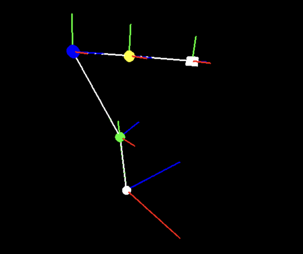
Figure 6 depicts the robotic arm as seen in the simulator, where inverse kinematics is run to determine the compatible joint angles. While running inverse kinematics, we specify and . We observe that if we provide a target pose within the arm’s available task space, the algorithm converges very quickly, taking between three and ten iterations to converge for all poses. However, one shortcoming of this model is that the user must correctly specify feasible target orientations along with the position in order to reach convergence, which is often cumbersome to determine in real life.
Arm Implementation
After retrieving the required arm configurations through inverse kinematics, we attempted to perform the task in real life using the robotic arm. The arm controls each joint through servos, and it receives power from an external Raspberry Pi connected to a DC power supply. The servos each accept input from 0° to 180°, so we accordingly renormalize our obtained values from inverse kinematics. When performing calculations, we additionally clamp the angles between this range after each iteration, which prevents us from receiving joint angles outside the capabilities of our servos. It is also important to note that the rest position of the arm pictured in Figure 4 is defined where each joint is at the middle of its range, so we also accounted for that when renormalizing.
However, attempting this task on the arm is a much more complicated task than running it on the simulator, as there exists many sources of error that we have failed to account for in the simulator. For instance, the starting position of the arm must be near perfect, as any slight shifts throw off the entire inverse kinematics calculations, resulting in a failed task. Additionally, with no ability to receive angular feedback from the servos or any way to sense the arm’s surroundings, we cannot dynamically adjust the angles to account for any discrepancies in positioning. As a result, we have found better success by manually controlling the arm, setting joint angles through trial and error. When doing this, we find that the task is indeed possible, if not tedious. Nonetheless, in theory, our calculations for inverse kinematics are correctly implemented and seem to behave correctly inside the 3D engine.